Generating distributions with the Stick Breaking version of the Dirichlet Process

Posted on 28 Jun 2018

The Dirichlet Process is a prior over distributions. The basic definition relays on measure theory and has some obscure definitions for most of people. Intuitevily, imagine we want to draw a distribution $G$ over the line of real numbers using some prior distribution $P$ . We say that $P$ is a Dirichlet Process if, for any possible partition of the line of real numbers, $(A_1, ..., A_m)$ , the probabilities over the partitions are distributed according to a Dirichlet distribution:

$G(A_1),...,G(A_m) \sim \text{Dirichlet}(\alpha(A_1),...,\alpha(A_k))$

There are different ways to generate a distribution G. One of the most popular is the Stick Breaking construction. The trick is to realize that

$G = \sum_k \pi_k \delta_{\theta_k}$

where $\pi_k$ weights sum up to 1, and the deltas are distributed around the line of the real numbers according to some distribution. The stick breaking construction goes as follows:

Take a stick of length 1 and make infinite random breaks. Each break removes a percentage $v_k$ of the remaining stick
$v_k \sim \text{Beta}(1, \alpha)$
The length of the removed break is
$\pi_k = v_k \prod_{i=1}^{k-1}(1-v_i)$
where $\prod_{l=1}^{k-1}(1-v_l)$ is the remaining length of the stick at step $k$ . At the end of the process we have a collection of segments whose length sum is 1.
Draw infinite samples from a base distribution $G_0$ :
$\phi_k \sim G_0$
where $G_0$ can be any distribution such as a Gaussian, a Poisson or a Multinomial.
We build our distribution as
$G = \sum_{k=1}^\infty \pi_k \delta_{\phi_k}$

Here is the R code to sample from a Dirichlet Process using the Stick Breaking construction:

library(dplyr)
library(ggplot2)

#'@title Stick Breaking construction of a Dirichlet Process
#'@param n number of samples
#'@param alpha concentration parameter
#'@param G0 base measure
DP_stick_breaking <- function(n, alpha, G0) {

  # Stick breaking
  v  <- rbeta(n, 1, alpha)
  
  pi <- numeric(n)
  pi[1] <- v[1] 
  pi[2:n] <- sapply(2:n, function(i) v[i] * prod(1 - v[1:(i-1)]))
  
  # Atoms from the base measure
  y <- G0(n) 
  return(list(atoms = y,
              pis = pi))
  # Sample from the Dirichlet Process G
  #theta <- sample(y, prob = pi, replace = TRUE)
  #return(theta)
}


# Choose a base distribution
G0 <- function(n) rpois(n, 7)       # Poisson
G0 <- function(n) rnorm(n, 0, 1)   # Gaussian

# Concentration parameter around the base distribution
alphas <- c(1, 10, 100, 1000)
n <- 1000
df.G <- as.data.frame(matrix(NA, 0, 4))
names(df.G) <- c("xp", "i", "atom", "pi")

df.samples <- as.data.frame(matrix(NA, 0, 4))
names(df.samples) <- c("xp", "i", "alpha", "samples")

for(alpha in alphas){
  for(xp in 1:3){
    cat("\n", alpha)
    
    # Generate a distribution from the DP(alpha, G0)
    G <- DP_stick_breaking(n, alpha, G0)
    df.G <- bind_rows(df.G, 
                      list(xp = rep(xp, n), 
                           alpha= rep(alpha, n), 
                           i=1:n,
                           atom = G$atoms,
                           pi=G$pis))
    
    # Generate samples from the DP
    samples <- sample(G$atoms, prob = G$pis, replace = TRUE)
    df.samples <- bind_rows(df.samples, 
                            list(xp = rep(xp, n), 
                                 alpha= rep(alpha, n), 
                                 i=1:n, 
                                 sample=samples))
  }
}

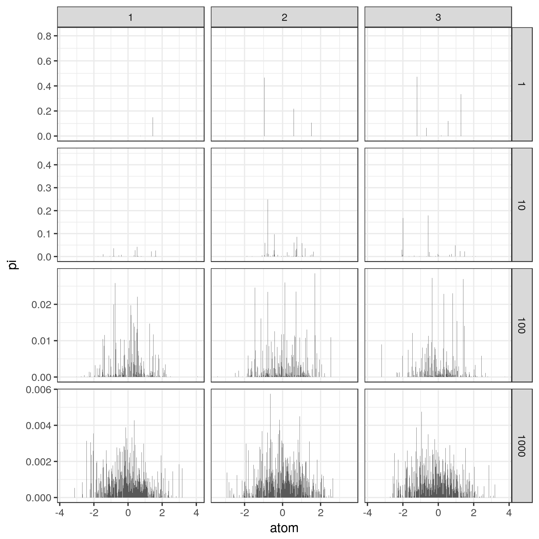
# Plot the distributon drawn by the DP
df.G$alpha <- factor(df.G$alpha)
p <- ggplot(df.G, aes(x=atom, y=pi)) + 
  geom_col(width=0.01)+
  facet_grid(alpha ~ xp, scales = "free") +
  theme_bw()
print(p)
ggsave(p, filename = paste0("fig15_DP.png"), 
       height=16, width=16, units='cm')

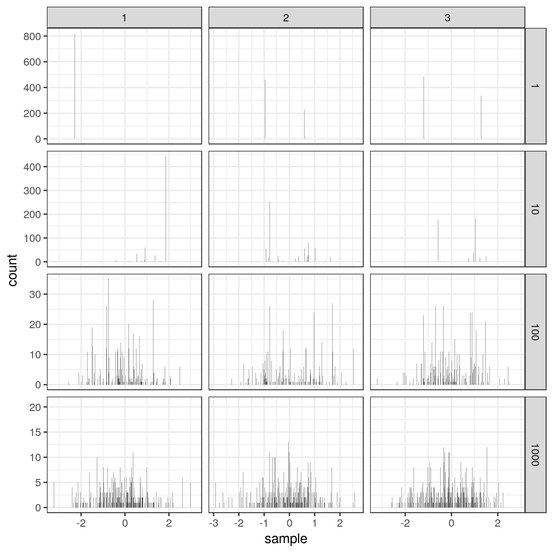
# Plot samples from the distribution
df.samples$alpha <- factor(df.samples$alpha)
p <- ggplot(df.samples, aes(x=sample)) + 
     #geom_density() +
     #geom_histogram(bins=100, aes(y=..count../sum(..count..))) +
     geom_histogram(bins=1000) + 
     facet_grid(alpha ~ xp, scales = "free") +
     theme_bw()
print(p)
ggsave(p, filename = paste0("fig16_DPsamples.png"), 
       height=16, width=16, units='cm')

And here are the results of Dirichlet Process $G$ generated with the Stick Breaking and different concentration $\alpha$ , and samples obtained from these $G$ :

Fig.1 - (Left) Distributions drawn from a Dirichlet Processes with different concentration parameters. (Right) Samples from these distributions. Columns represent repetitions of the experiment.