The curse of dimensionality
The curse of dimensionality is the effect by which many mathematical problems become hard when we deal with many dimensions. In this note we explain why, in high dimensions, a box with a melon inside contains more air than melon, why life gets complicated with many dimensions, and some of the effects of the curse in statistics and machine learning.
Multidimensional flies
Minsky is a one-dimensional robot that lives in a universe contained in a segment of 1 metre. One day the robot sees a fly flying back and forth along the segment. Minsky decides to catch it with his fly swatter, which has a length of \(l = 0.8\). Since Minsky has no idea where the fly will be at any given moment, he swings the swatter at random. The probability of catching the fly equals the fraction of space he can cover with his swatter:
\[p = \frac{l}{1} = 0.8\]
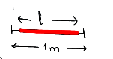
Now imagine that Minsky lives in a two-dimensional space, a plane of 1 m \(\times\) 1 m, and that his swatter is 0.8 m \(\times\) 0.8 m. The probability of catching the fly is now:
\[p = \frac{l^2}{1} = 0.8^2\]
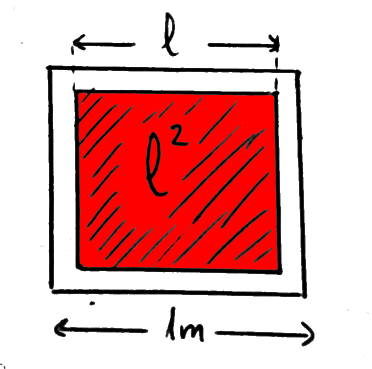
Curious. The fly’s safe zone takes up more and more room, at the expense of the space covered by the swatter. In fact, if we keep adding dimensions, the probability of catching the fly in \(d\) dimensions is:
\[p = l^d\]The plot shows how this probability fades away as the number of dimensions grows.
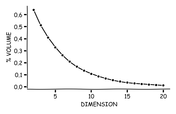
It looks like in high dimensions there is no way to catch a fly!
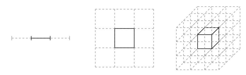
This picture shows the same idea. As we add dimensions, the highlighted segment (the swatter) is a smaller and smaller part of the whole, and the fly has more and more room to roam free:
Multidimensional leaks
On to a second example, where we play with spheres instead of cubes. Imagine our living room, 1 m \(\times\) 1 m, has leaks all over the ceiling, and we want to collect as much water as possible. So we put down a basin of 1 m in diameter. The fraction of water that falls inside the basin is the ratio between the surface of the basin and the surface of the room. That is:
\[p = \frac{\pi R^2}{1} = \frac{\pi 0.5^2}{1} = \frac{\pi}{4} \approx 0.78\]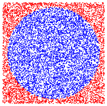
So only 22% of the water falls outside (red dots).
What happens in \(d\) dimensions?
\[p = \frac{ \frac{\pi^{d/2}}{\Gamma(\frac{d}{2} +1)}R^d}{1} = \frac{\pi^{d/2}}{\Gamma(\frac{d}{2} +1)}R^d\]where the numerator is the volume of a sphere of radius \(R\).
Looking at the plot, we see that from dimension 4 on, more water falls outside than inside!
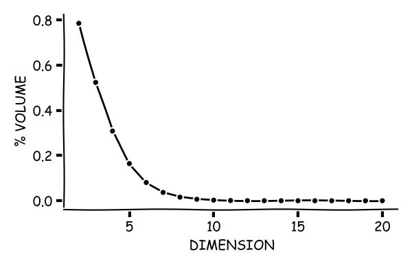
Back to the melon in a box: the more dimensions the box has, the more air and the less melon.
Darts, football and multidimensional aim in general
This difficulty of aiming in high dimensions shows up everywhere. On a multidimensional dartboard, the probability of hitting the bullseye (unless we enlarge it) goes to zero. The same happens in football with the probability of scoring a goal (unless we make the goal bigger as we add dimensions). And in basketball, the probability of scoring a basket vanishes too.
Doing sports in high dimensions is very, very boring.
Machine learning: deserted spaces and empty neighbourhoods
In machine learning the problem goes like this. Imagine I am given a list of animals described by their weight and height, and a label that says whether each animal is a cat or a dog. For simplicity, let us assume each attribute takes three possible values: low, medium, high. The number of possible combinations is:
\[3~\text{weights} \times 3~\text{heights} = 3^2\]With a few dozen examples I will start to see which combinations of attributes tend to be dogs and which tend to be cats.
Now, to improve my classifier, I am given four more attributes: ear size, tail length, amount of fur, and hours of sleep… It sounds useful, but if I am not given more examples, nobody is doing me any favours. My space has grown brutally! The number of combinations is now:
\[3~\text{weights} \times 3~\text{heights} \times ~ ... = 3^6\]Before I had 9 possible combinations; now there are 729. The problem is that if I only get 10 examples, most combinations are left unexplored.
So in high dimensions, everything is far from everything. This brings an extra problem: the notion of neighbourhood (closeness in the attributes, that is, being similar), so useful in learning, disappears. If everything is far from everything, a point has no neighbours (similar points) and I cannot tell whether it is a cat or a dog. “But the neighbourhood is defined arbitrarily, let us make its radius bigger!”, some will say. The problem is that if the radius is very large, everybody ends up being everybody’s neighbour, which is as useless as nobody being anybody’s neighbour.
In short, adding dimensions turns my space into a desert, a multidimensional Mad Max.
There are two ways out: use fewer attributes, or get more examples.
Probability distributions: typical sets
The curse of dimensionality also affects probability distributions (Gaussian, Poisson, etc.): the mode stops being interesting.
The mode of a distribution is the point of highest probability density. However, rather than density, what we really care about is mass, computed as density times volume (see picture):
\[\text{mass} = \text{density} \times \text{volume}\]
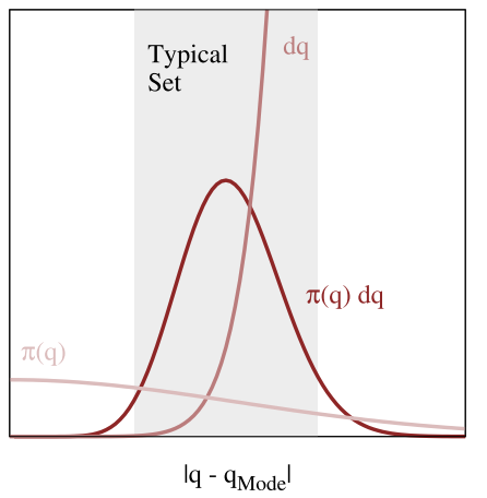
The picture shows a (made-up) example of density (\(\pi(q)\)), volume (of each little piece of space, \(dq\)) and their product. Let us see what happens with two of the best-known distributions: the Uniform and the Gaussian.
- Uniform distribution
We already met the uniform distribution implicitly, with the leaks: given a floor of \(d_1 \times d_2\), drops are equally likely to fall anywhere on it. We saw that, as we added dimensions, most drops fell near the edges of the floor. In other words, a drop is more likely to land somewhere near the edge than right in the centre.
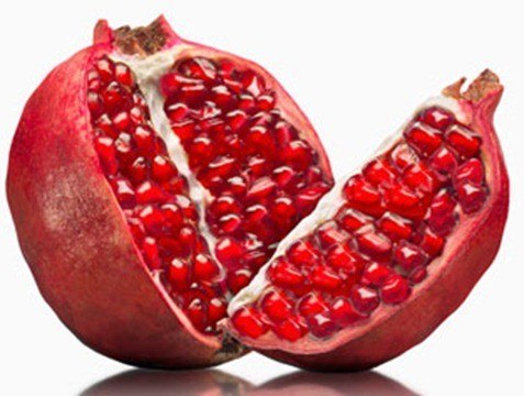
Think of a pomegranate. Imagine we pick its seeds from the outside in, turning the pomegranate in our hands. The first turns will give us more seeds than the last ones!
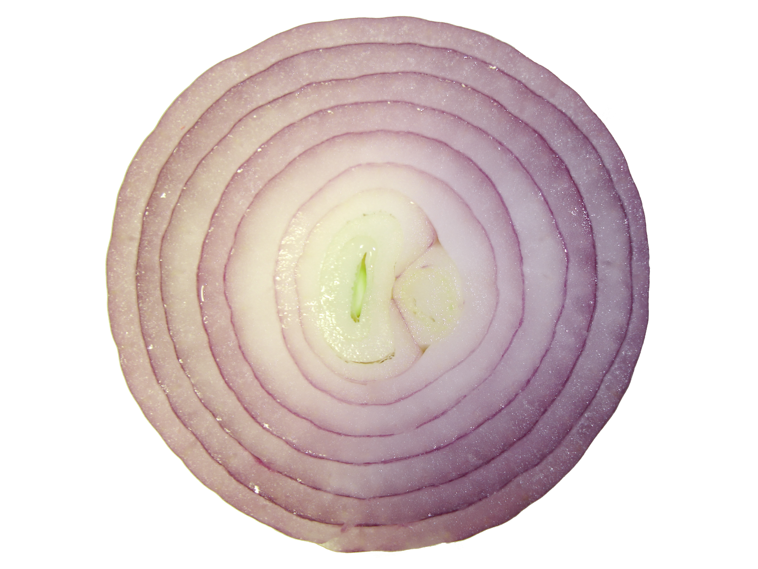
Or an onion, which is also uniformly dense and whose outer layers have more mass than the inner ones:
The uniform distribution gives the same probability density to every point of the space. As we move away from the centre, the volume grows and the density stays the same, so the farther from the centre, the larger the mass. Hence the leaks falling outside the basin rather than inside.
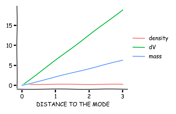
With many dimensions, the volume grows faster as we move away from the mode, and so does the mass, since the density is constant.
- Gaussian distribution
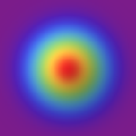
What if the leaks followed a Gaussian shape on the ceiling? The volume grows as we move away from the centre, but the density goes down. The region that collects the most water is given by the product of the two.
In two dimensions, the mass already starts to shift away from the centre. Where is most of it?
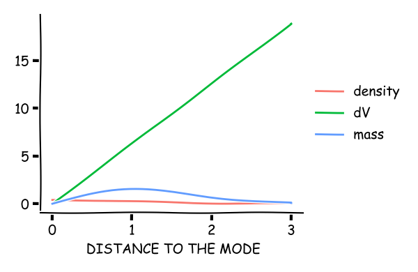
As before, in many dimensions the volume grows faster as we move away from the mode. For the Gaussian, the effect is that the little hill marking the region with the most mass (known as the typical set) moves farther and farther to the right, divorcing itself from the mode. For a standard Gaussian in \(d\) dimensions, almost all the mass sits in a thin shell at distance \(\approx \sqrt{d}\) from the mode, and almost none near the mode itself.
This is why, when there are many variables, the mode is a poor summary of the distribution: what matters are expectations, which integrate over the mass, and that is why methods like MCMC try to explore the typical set rather than climb to the mode.
Conclusion
The curse of dimensionality is a phenomenon that affects many mathematical problems. Geometrically, it can be summed up as a melon in a multidimensional box, where there is more air than melon.
In statistics and machine learning, adding variables to a problem can look like a good idea but, if it does not come with more observations, it can make things worse and turn our space into a desert where learning and statistical inference get harder.