Non-negative Matrix Factorization (Lee and Seung algorithm)

Posted on 03 Sep 2018

Introduction

Nonnegative Matrix Factorization (NMF) is a technique that tries to approximate a nonnegative matrix V (with $F \times N$ dimensions) into the product of two smaller (also nonnegative) matrices $W (F \times K)$ and $H (K \times N)$.

For those familiar with PCA, NMF is a sort of PCA with nonnegative (and therefore more easy to interpret by humans) basis. Moreover, these basis do not need to be orthogonal.

One of my favorite applications of NMF is in recomender systems. If $V$ contains some ratings of users to movies ($F$ users and $N$ movies), $W$ will contain the atraction of a each user to each topic, and H will contain the amount of each topic in each movie. This decomposition is a compressed version of the original matrix. Moreover, once we have this information we can easily guess, by a simple multiplication, the rating of a user to an unrated movie.

Implementing a NMF algorithm

The first NMF algorithm was derived by Lee and Seung. The thing is that, before deriving our NMF algorithm, we have to choose a distance metric to assess the quality of the approximation

\begin{equation} V \approx W H \end{equation} Lee and Seung considered two cost functions. The Euclidean and the generalized Kullback-Leiberg (KL), also known as the I-divergence. In this post we will work with the (generalized) KL divergence. We want to find the decomposition that minimizes the KL divergence

\begin{equation} \underset{W,H}{\operatorname{argmin}} D_{KL}(V || WH) \end{equation} where the KL divergence is defined as

\begin{equation} D_{KL}(A || B) = \sum_{ij} \left( A_{ij} \log \frac{A_{ij}}{B_{ij} } - A_{ij} + B_{ij}\right) \end{equation} The idea is to optimize W given H, then H given W and so on until the algorithm converges. A typical option is Gradient Descent, but convergence can be slow. Instead, Lee and Seung proposed Minorize-Maximization (MM) strategy. The idea of MM is to use an auxiliary function. We say that $G(h, h′)$ is an auxiliary function of $F(h)$ if $G(h, h′)$ is equal or greater than $F(h)$ everywhere and $G(h, h)=F(h)$. Note that, when the first parameter is fixed $G(h, h′)$ is a curve. The first parameter tell us the point where it touches $F$. If we can design such a function, we can find the $h_{min}$ at each step and then updating the curve to $G(h_{min}, h′)$ until we reach a minimum.

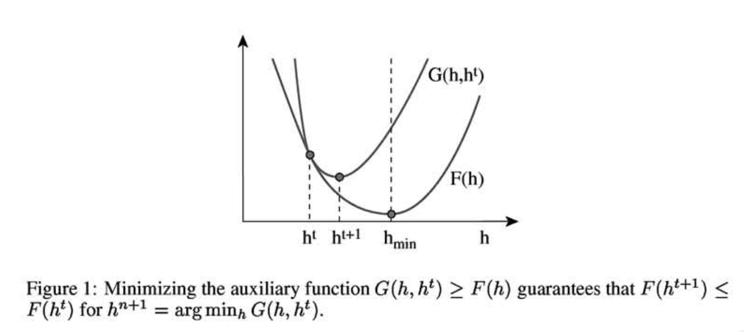
In our case, $F(h)$ is a KL divergence. In their paper, Lee and Seung provide an auxiliary function which can be easily minimized. Doing this for $W$ and $H$ they obtain the classic NMF updates:

Recall that the updates are supposed to minimize the KL divergence between the approximation and the true matrix. To monitorize this, let us code an R function that computes the KL divergence:

#' @title Compute the KL divergence (fast version)
#' @param A first matrix
#' @param B second matrix
#' @details This function is useful for debugging
KL_divergence_Lee <- function(A, B){
  eps <- 1e-6
  sum(A*log((A + eps)/ (B + eps)) - A + B)
}

Now we can write the algorithm, which iteratively updates W and H until convergence:

#' @title NMF with Lee and Saung multiplicative updates
#' @param V matrix to factorize
#' @param K number of latent factors (or dimensions)
#' @param W initial W matrix
#' @param H initial H matrix
#' @param maxiters maximum number of iterations
#' @details The number of iterations is set to maxiters.
nmf_Lee <- function(V, K, W, H, maxiters = 100){
  F <- nrow(V)
  N <- ncol(V)
  eps = 1e-05
  
  unit_f <- matrix(1, ncol=1, nrow=F)
  unit_n <- matrix(1, ncol=1, nrow=N)
  
  KLlog <- rep(NA, maxiters)
  for (i in 1:maxiters){
    cat("\n iteration:", i, "/", maxiters)

    # update W (matricial)
    # matlab: W = W .* ((V./(W*H + options.myeps))*H')./(ones(m,1)*sum(H'));
    W <- W * ((V / (W%*%H + eps)) %*% t(H)) / (unit_f %*% rowSums(H))
    
    # update H (matricial)
    # matlab: H = H .* (W'*(V./(W*H + options.myeps)))./(sum(W)'*ones(1,n));
    H <- H * (t(W) %*% (V / (W%*%H + eps))) / (colSums(W) %*% t(unit_n))
    
    # Trace KL divergence
    KLlog[[i]] <- KL_divergence_Lee(V, W%*%H)
  }
  list(W=W, H=H, KLlog = KLlog)
}

Faces dataset

To play with our code, let us download the ATT Faces dataset. The dataset consists of 10 black and white photos of each member of a group 40 individuals. 400 images in total.

library(pixmap)

url <- "http://www.cl.cam.ac.uk/Research/DTG/attarchive/pub/data/att_faces.zip"
filename <- basename(url)
download.file(url = url, destfile = filename)
unzip(filename, exdir = "faces")
dirname <- './faces/'
dirs <- list.dirs("./faces")
files <- list.files(pattern = ".pgm", recursive = TRUE)
V <- matrix(nrow = 92*112, ncol = length(files))
for (i in 1:length(files)){
  v <- read.pnm(file = files[i], cellres=1)
  V[,i] <- floor(as.vector(v@grey)*255)
}


#'@title Plot a face
#'@details Given a vectorized image, reconstruct its matrix and plot it
plot_face <- function(arr10304, col=gray(0:255/255)){
  m <- matrix(arr10304, ncol=92,  nrow = 112)
  image(t(m[112:1,]), asp=112/92, axes = FALSE, col=col)
}

# Plot some faces
par(mfrow=c(10,20), mar=c(0, 0.2, 0, 0), oma=c(0,0,0,0))
for(i in sample(400,200)){
  plot_face(V[,i])
}

Now we call our NMF algorithm using this dataset as input. Let say we want to use $K=100$ latent dimensions, or dictionary basis.

F <- nrow(V)
N <- ncol(V)
K = 100
W <- matrix(rpois(n = F*K, lambda = 10), nrow = F, ncol = K) 
H <- matrix(rpois(n = N*K, lambda = 10), nrow = K, ncol = N) 
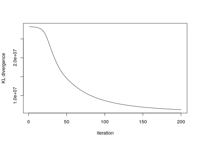
res <- nmf_Lee(V, K, W, H, maxiters = 200)

Did the algorithm convergence? The KL divergence is improving slowly after 200 iterations, so we will stop here.

plot(res$KLlog, type='l', ylab= "KL divergence", xlab = "iteration")

Let’s see how does our dictionary look like, and let’s compare with the dictionary of a PCA:

# PCA 
pca   <- prcomp(V)
V_hat_pca  <- pca$x[,1:K] %*% t(pca$rotation[,1:K])

# Plot some faces and their reconstrctions
par(mfrow=c(10,20), mar=c(0, 0.2, 0, 0), oma=c(0,0,0,0))
for(k in 1:100){
  plot_face(res$W[,k], col = heat.colors(255))
}
for(k in 1:100){
  plot_face(pca$x[,k], col = heat.colors(255))
}

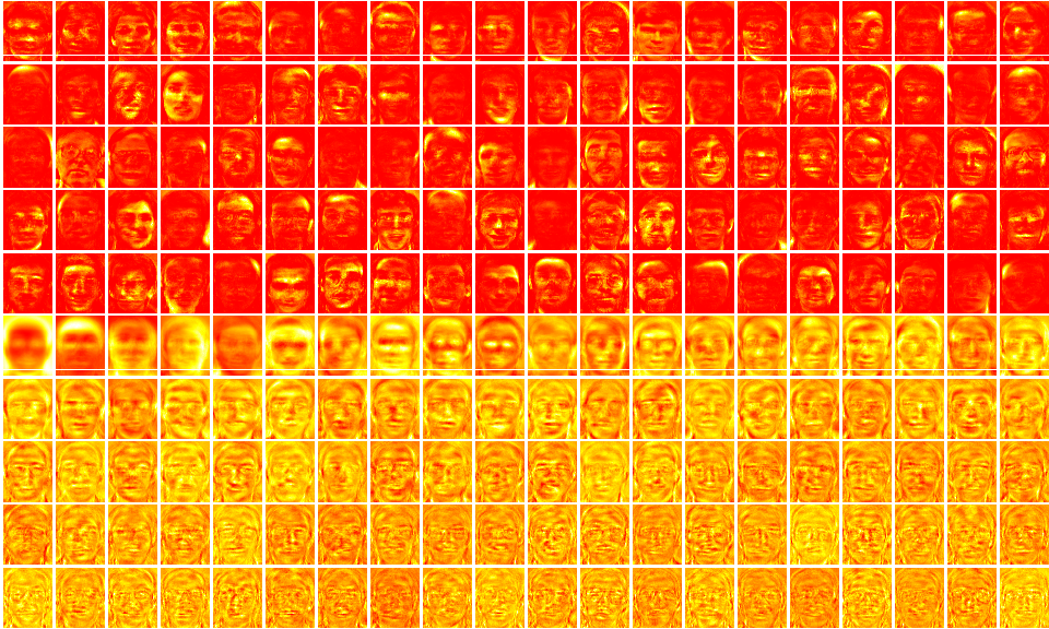Dictionaries obtained with NMF (above) and PCA (below)

Note that, while PCA tends to create “holistic” bases, NMF prefers bases that focus on different parts of the face, which makes NMF more easy to interpret. Finally, let’s see how good the reconstruction is, and let us compare with a PCA:

# PCA
mu    <- colMeans(V)
pca   <- prcomp(V)
Kpca <- K
V_hat_pca  <- pca$x[,1:Kpca] %*% t(pca$rotation[,1:Kpca])
V_hat_pca  <- scale(V_hat_pca, center = -mu, scale = FALSE)

# NMF reconstruction
V_hat <- res$W %*% res$H

# Plot some faces and their reconstructions
par(mfcol=c(3,10), mar=c(0,1,0,0), oma=c(0,0,0,0))
for(i in sample(ncol(V),10)){
  plot_face(V[,i])
  plot_face(V_hat[,i])
  plot_face(V_hat_pca[,i])
}

Reconstructions obtained with NMF (above) and PCA (below)

Note that the quality of our reconstruction depends on the chosen number of latent dimensions or components $K$ (the larger, the more expressive our dictionary basis), the convergence (we can try a bunch more of iterations) and the quality of the model to the data (KL is appropiate for Poisson data, PCA for Gaussian data).

Final remarks

The algorithm presented in this post was the one who triggered the interested in NMF in 1999. However, the story continued for the next years and until today, taking different research avenues.

In one of these avenues researchers proposed NMF algorithms to minimize other cost functions and assuming other likelihoods beyond Poisson and Gaussian. At some point, someone realized that there are some conections between cost functions and likelihoods: for instance, the KL minimization in this post is equivalent to find the MLE estimator assuming our data come from a Poisson distribution with mean $WH$.

On the probabilistic side, Bayesians consider $W$ and $H$ as random latent variables, and instead of trying to find point extimators for $W$, $H$ they infer a posterior distribution over each of them.

Finally, scalability is another important issue nowadays: people are playing with optimization algorithms that use a subsample of the data at each iteration (Stochastic Gradient Descent, Stochastic Variational Inference…) so that iterations are computationally cheaper while keeping good convergence properties in terms of number of iterations.