Biased and unbiased estimators
Posted on 20 Jul 2018
Introduction
In statistics, we often hear that an estimator is biased or unbiased. In this post, I will introduce the definition of bias and then I will work through a couple of examples (with R code!). I will always consider that we want to approximate an expectation, since this is a very common problem in Machine Learning. However, the same ideas can be applied to estimations of other quantities (e.g.: higher moments such as variances).
Biased and unbiased estimators
Imagine we have a population of N individuals. If we have access to all the individuals and their data, we can compute associated quantities such as their mean height and weight, their median salary, or the age of the older individual. Each of these quantities, denoted as θ is computed as a function f that takes the N individuals as input and returns a quantity. Unfortunatelly, often we cannot access to all the individuals, but to S samples of the population. An estimator is a function $\\hat{\\theta}(x\_1,…x\_S)$ that, taking a subset of individuals, tries to estimate the real quantity θ, i.e.:
\begin{align} \hat{\theta}(\mathbf{x}_S) \approx \theta \end{align} The estimator $\\hat{\\theta}$ is a random variable because, while it is a (deterministic) function, it is applied over a random sample xS. Among the different properties of our estimator, one the most important is the bias, defined as
\begin{align} \mathbb{E}[\hat{\theta}] - \theta \end{align} If this difference is zero, then we say that the estimator is unbiased. Else, the estimator is biased.
Estimator of a mean
Imagine that we have random variable X with N possible outcomes, denoted as x_1,…,x_N. Each outcome has a probability p(x_1),…p(x_N). The expectation of the random variable is defined as:
\begin{align} \mathbb{E}[x] = \sum_{n=1}^N x_n p(x_n) \end{align} The expectation is just the weighted sum of the outcomes, where the weights are given by the probability of each outcome x_n. The expectation is a deterministic value, not random, since it is a deterministic measure over the whole population.
In most cases, however, we do not have access to the probability distribution p(xn) and instead we are given samples of the original population according to that distribution:
\begin{align} x_s \sim p(x) \end{align} The question is whether we can propose an unbiased estimator of the real expectation. The classic estimator of a mean is the sample mean, that is:
\begin{align} \hat{\theta} = \frac{1}{S}\sum_s x_{s} \end{align} We can easily checked that this estimator is unbiased:
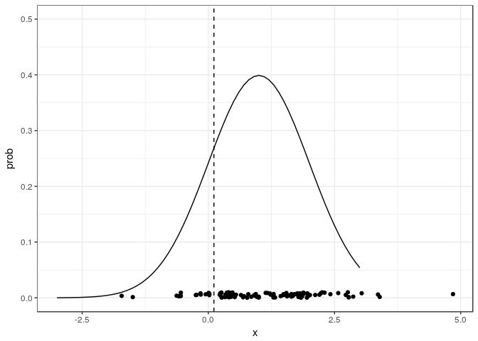
\begin{align} \mathbb{E}[\hat{\theta}] = \mathbb{E}[\frac{1}{S}\sum_s x_{s}] = \frac{1}{S}\sum_j \mathbb{E} [x_s] = \frac{1}{S} \mathbb{E} [x_s] = \mathbb{E} [x] \end{align} Let’s play with a toy example where our variable comes from a Gaussian distribution centered at 1. We will plot the true distribution, the samples used for the estimator, and the value of the estimator.
# Estimate the mean of a Gaussian random variable
# given a random sample of size S

library(tidyr)
library(ggplot2)

estimator <- function(samples){
  mean(x_samples)
}

S <- 100
mu <- 1
sdev <- 1
x           <- seq(-3,3, by=0.1)
prob        <- dnorm(x, mean = mu, sd = sdev)

# Estimate once
x_samples   <- rnorm(n = S, mean = mu, sd = sdev)
theta_hat   <- estimator(x_samples)

df.pdf <- data.frame(x = x, prob = prob)
df <- data.frame(x = x_samples, prob = runif(S)/100)
ggplot(df, aes(x = x, y = prob)) +
  geom_point() +
  geom_line(data = df.pdf, aes(x=x, y=prob))+
  geom_vline(aes(xintercept = theta_hat), linetype = 2) +
  ylim(c(0,0.5))+
  theme_bw()

Sample points from an infinite population, and its estimated mean. The curve shows the true underlying distribution, with its mean in zero.
It looks unbiased, but is this real? That is, will my estimator move around the true mean value if I repeat the experiments (with different samples) many times?
# Estimate many times to analyze bias
n_reps <- 10000
theta_hat_samples <- rep(NA, n_reps)
for(xp in 1:n_reps){
  x_samples   <- rnorm(n = S, mean = mu, sd = sdev)
  theta_hat   <- estimator(x_samples)
  theta_hat_samples[xp]  <- theta_hat
}

# Empirical bias
bias <- cumsum(theta_hat_samples) / seq_along(theta_hat_samples) - mu
df.bias <- data.frame(bias = bias, repetitions = 1:length(bias))
ggplot(df.bias, aes(x=repetitions, y = bias)) + geom_line() + theme_bw()
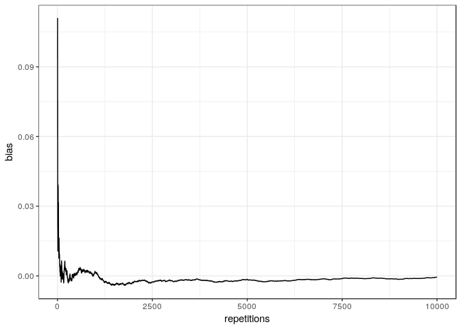 Evolution of the empirical bias with the number of repetitions of the
experiment
Evolution of the empirical bias with the number of repetitions of the
experiment
The figure shows empirically that the more we repeat the experiment, the more the average of our estimator converges to the true value (the distance to the true value decreases).
Estimation of the log of the mean
Imagine now that we want to estimate the log of the expectation log𝔼 *x* , defined as
\begin{align} \log \mathbb{E}[x] = \log\left( \sum_{n=1}^N x_n p(x_n) \right) \end{align} and that once we got some samples we approximate this as
\begin{align} \hat{\theta} = \log \big(\frac{1}{S}\sum_s x_s\big) \end{align} And now let’s see whether it is biased or unbiased (we will use Jensen’s inequality):
\begin{align} \mathbb{E}[\hat{\theta}] = \mathbb{E}\big[ \log \big(\frac{1}{S}\sum_s x_s\big)\big] \leq \log \mathbb{E}\big[\frac{1}{S}\sum_j x_s\big] = \log \mathbb{E}[x] \end{align} This estimator is biased and, more specifically, it underestimates the true value. Note, however, that the equality in the middle of the equation holds when the inside term is not a random variable but a constant, which happens if we take the entire population. That means that, the larger the population sample, the smaller the bias.
Let’s repeat the experiments with our new estimator. Note that now the true value is the log of the mean, hence 0.
# Estimate the mean of a Gaussian random variable
# given a random sample of size S

library(tidyr)
library(ggplot2)

estimator <- function(samples){
  log(mean(x_samples))
}

S <- 100
mu <- 1
sdev <- 1
x           <- seq(-3,3, by=0.1)
prob        <- dnorm(x, mean = mu, sd = sdev)

# Estimate once
x_samples   <- rnorm(n = S, mean = mu, sd = sdev)
theta_hat   <- estimator(x_samples)

df.pdf <- data.frame(x = x, prob = prob)
df <- data.frame(x = x_samples, prob = runif(S)/100)
ggplot(df, aes(x = x, y = prob)) +
  geom_point() +
  geom_line(data = df.pdf, aes(x=x, y=prob))+
  geom_vline(aes(xintercept = theta_hat), linetype = 2) +
  ylim(c(0,0.5))+
  theme_bw()
 Probability density, some samples from it and the estimator of the log
of the mean
Probability density, some samples from it and the estimator of the log
of the mean
Finally let’s see what happens if we repeat the experiment many times.
# Estimate many times to analyze bias
n_reps <- 10000
theta_hat_samples <- rep(NA, n_reps)
for(xp in 1:n_reps){
  x_samples   <- rnorm(n = S, mean = mu, sd = sdev)
  theta_hat   <- estimator(x_samples)
  theta_hat_samples[xp]  <- theta_hat
}

# Empirical bias
bias <- cumsum(theta_hat_samples) / seq_along(theta_hat_samples) - log(mu)
df.bias <- data.frame(bias = bias, repetitions = 1:length(bias))
ggplot(df.bias, aes(x=repetitions, y = bias)) + geom_line() + theme_bw()
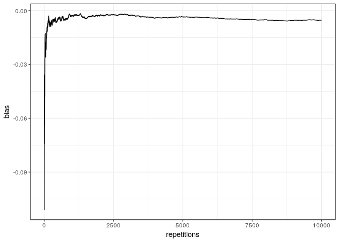 Evolution of the empirical bias with the number of repetitions of the
experiment
Evolution of the empirical bias with the number of repetitions of the
experiment
Indeed, it confirms that the estimator is biased and underestimates the true value.
Final remarks
We have seen the definition of a biased / unbiased estimator and we have applied this to estimation of the mean. There are other properties of the estimators that are important, such as its variance, its consistence, but these are out of the scope of this post.
Estimating the log of the mean can be pointless, but it has some real applications. In this recent paper, for instance, the authors deal with something like
\begin{align} \log \mathbb{E}_q\big[ \left(\frac{p(\theta, X)}{q(\theta | X)}\right)^{1-\alpha} \big] \approx \log \frac{1}{K}\sum_k \big[ \left(\frac{p(\theta_k, X)}{q(\theta_k | X)}\right)^{1-\alpha} \big] \end{align} Following the same reasoning than above, one can see that this approximation biased. In the paper, the authors are at least able to characterize the amount of bias introduced.
References
Here there are a couple of links with basic material: